Introduction
After conducting an MAIC, the results can be effectively illustrated through visual representations of the weighted and non-weighted data. This can be achieved by plotting Kaplan-Meier (KM) curves and comprehensively depicting the time-to-event data. To generate these curves, it is crucial to obtain pseudo-IPD from the comparator study through the digitization of KM curves from the comparator study. For guidance on this process, refer to the works of Guyot et al. and Liu et al. [1,2]
Unanchored case
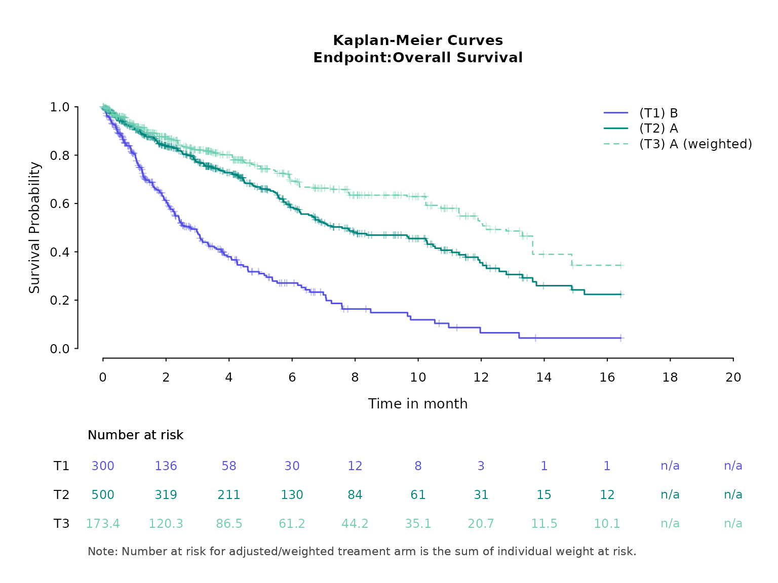
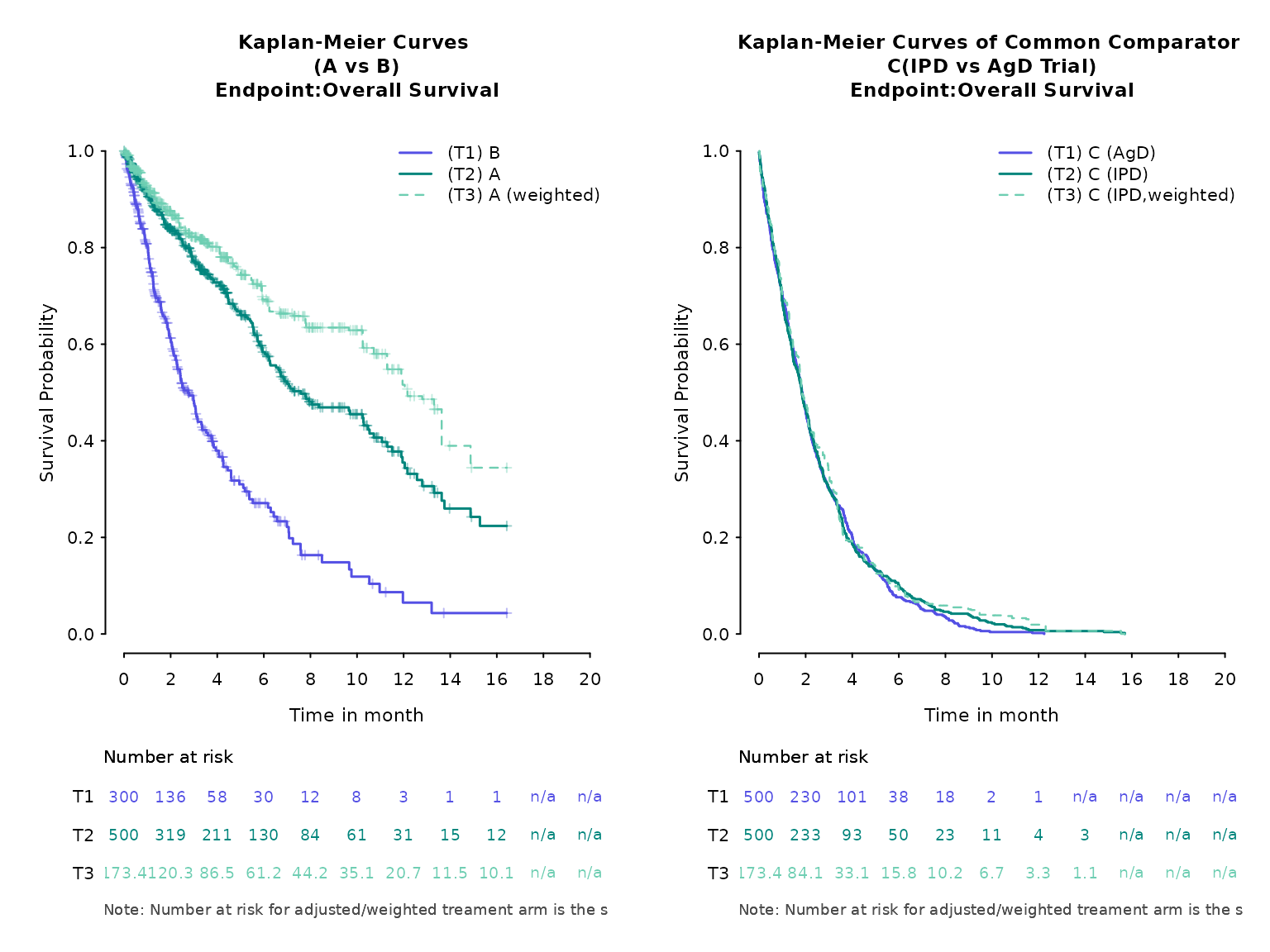
Here is a Kaplan-Meier plot using base R graphics. Note that number at risk for weighted treatment arm is the sum of individual weights at risk. Consequently, number at risk for weighted treatment arm at time 0 is different from calculated ESS or original sample size. One can modify this by using normalized weights instead. If we use normalized weights, weights are in the original unit scale and so number at risk at time 0 is equal to the sample size.
Another important thing to note is that the time input that we
specify (i.e. adtte_sat in our example) should be in days.
time_scale component allows us to change days into the
analysis unit of preference.
kmplot(
  weights_object = weighted_sat,
  tte_ipd = adtte_sat,
  tte_pseudo_ipd = pseudo_ipd_sat,
  trt_ipd = "A",
  trt_agd = "B",
  trt_common = NULL,
  normalize_weights = FALSE,
  endpoint_name = "Overall Survival",
  km_conf_type = "log-log",
  time_scale = "month",
  time_grid = seq(0, 20, by = 2),
  use_colors = NULL,
  use_line_types = NULL,
  use_pch_cex = 0.65,
  use_pch_alpha = 100
)
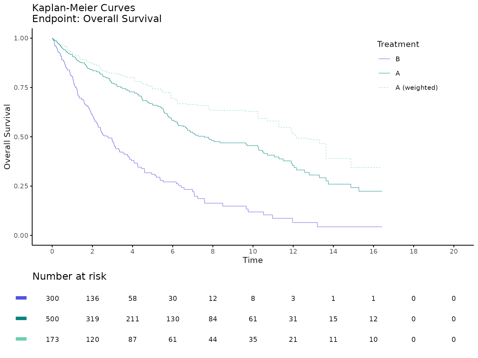
There is also a ggplot option for Kaplan-Meier curves using
survminer R package.
kmplot2(
  weights_object = weighted_sat,
  tte_ipd = adtte_sat,
  tte_pseudo_ipd = pseudo_ipd_sat,
  trt_ipd = "A",
  trt_agd = "B",
  trt_common = NULL,
  normalize_weights = FALSE,
  endpoint_name = "Overall Survival",
  km_conf_type = "log-log",
  time_scale = "month",
  break_x_by = 2,
  xlim = c(0, 20),
  censor = FALSE
)
Anchored case
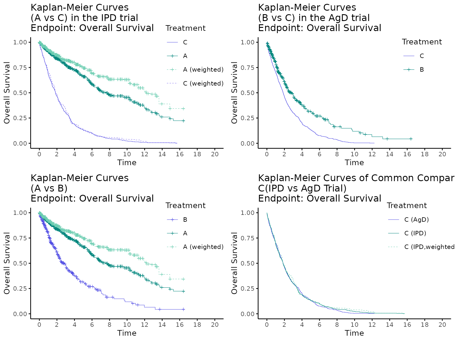
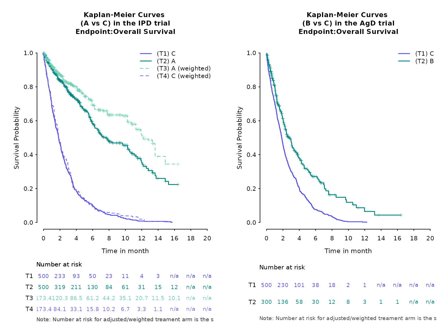
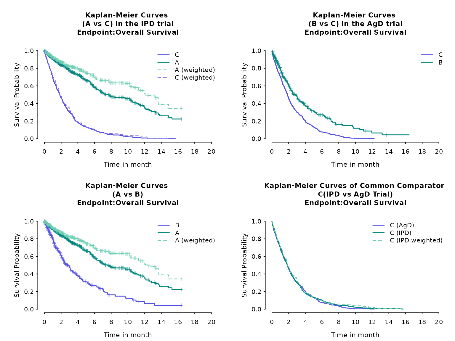
Here is an example for an anchored case.
data(weighted_twt)
data(adtte_twt)
data(pseudo_ipd_twt)

# plot by trial
kmplot(
  weights_object = weighted_twt,
  tte_ipd = adtte_twt,
  tte_pseudo_ipd = pseudo_ipd_twt,
  trt_ipd = "A",
  trt_agd = "B",
  trt_common = "C",
  normalize_weights = FALSE,
  endpoint_name = "Overall Survival",
  km_conf_type = "log-log",
  km_layout = "by_trial",
  time_scale = "month",
  time_grid = seq(0, 20, by = 2),
  use_colors = NULL,
  use_line_types = NULL,
  use_pch_cex = 0.65,
  use_pch_alpha = 100
)
# plot by arm
kmplot(
  weights_object = weighted_twt,
  tte_ipd = adtte_twt,
  tte_pseudo_ipd = pseudo_ipd_twt,
  trt_ipd = "A",
  trt_agd = "B",
  trt_common = "C",
  normalize_weights = FALSE,
  endpoint_name = "Overall Survival",
  km_conf_type = "log-log",
  km_layout = "by_arm",
  time_scale = "month",
  time_grid = seq(0, 20, by = 2),
  use_colors = NULL,
  use_line_types = NULL,
  use_pch_cex = 0.65,
  use_pch_alpha = 100
)
# plot all
kmplot(
  weights_object = weighted_twt,
  tte_ipd = adtte_twt,
  tte_pseudo_ipd = pseudo_ipd_twt,
  trt_ipd = "A",
  trt_agd = "B",
  trt_common = "C",
  normalize_weights = FALSE,
  endpoint_name = "Overall Survival",
  km_conf_type = "log-log",
  km_layout = "all",
  time_scale = "month",
  time_grid = seq(0, 20, by = 2),
  use_colors = NULL,
  use_line_types = NULL,
  use_pch_cex = 0.65,
  use_pch_alpha = 100
)
Again there is a ggplot option
data(weighted_twt)
data(adtte_twt)
data(pseudo_ipd_twt)

# plot all
kmplot2(
  weights_object = weighted_twt,
  tte_ipd = adtte_twt,
  tte_pseudo_ipd = pseudo_ipd_twt,
  trt_ipd = "A",
  trt_agd = "B",
  trt_common = "C",
  normalize_weights = FALSE,
  endpoint_name = "Overall Survival",
  km_conf_type = "log-log",
  km_layout = "all",
  time_scale = "month",
  break_x_by = 2,
  xlim = c(0, 20),
  show_risk_set = FALSE
)