Illustration using example data
This example reads in centered_ipd_twt data that was
created in calculating_weights vignette and uses
adtte_twt and pseudo_ipd_twt datasets to run
survival analysis using the maic_anchored function by
specifying endpoint_type = "tte".
Set up is very similar to unanchored_survival vignette,
except now that we have a common treatment between two trials. Common
treatment has to have same name in the data and we need to specify
additional parameter, trt_common, in
maic_unanchored.
data(centered_ipd_twt)
data(adtte_twt)
data(pseudo_ipd_twt)

centered_colnames <- c("AGE", "AGE_SQUARED", "SEX_MALE", "ECOG0", "SMOKE", "N_PR_THER_MEDIAN")
centered_colnames <- paste0(centered_colnames, "_CENTERED")

#### derive weights
weighted_data <- estimate_weights(
  data = centered_ipd_twt,
  centered_colnames = centered_colnames
)

# inferential result
result <- maic_anchored(
  weights_object = weighted_data,
  ipd = adtte_twt,
  pseudo_ipd = pseudo_ipd_twt,
  trt_ipd = "A",
  trt_agd = "B",
  trt_common = "C",
  normalize_weight = FALSE,
  endpoint_name = "Overall Survival",
  endpoint_type = "tte",
  eff_measure = "HR",
  time_scale = "month",
  km_conf_type = "log-log"
)
There are two summaries available in the result: descriptive and
inferential. In the descriptive section, we have summaries from fitting
survfit function. Note that restricted mean (rmean),
median, and 95% CI are summarized in the time_scale
specified.
result$descriptive$summary## trt_ind treatment type records n.max n.start events
## 1 C C IPD, before matching 500 500.0000 500.0000 500.00000
## 2 A A IPD, before matching 500 500.0000 500.0000 190.00000
## 3 C C IPD, after matching 500 199.4265 199.4265 199.42645
## 4 A A IPD, after matching 500 199.4265 199.4265 65.68877
## 5 C C AgD, external 500 500.0000 500.0000 500.00000
## 6 B B AgD, external 300 300.0000 300.0000 178.00000
## events% rmean se(rmean) median 0.95LCL 0.95UCL
## 1 100.00000 2.564797 0.11366994 1.836467 1.644765 2.045808
## 2 38.00000 8.709690 0.35514766 7.587627 6.278691 10.288538
## 3 100.00000 2.447736 0.17380451 1.786772 1.327555 2.200695
## 4 32.93885 10.166029 0.54999149 11.900015 7.815275 14.873786
## 5 100.00000 2.455272 0.09848888 1.851987 1.670540 2.009650
## 6 59.33333 4.303551 0.33672602 2.746131 2.261125 3.320857
# Not shown due to long output
# result$descriptive$survfit_ipd_before
# result$descriptive$survfit_ipd_after
# result$descriptive$survfit_pseudo
In the inferential section, we have the fitted models stored
(i.e. survfit and coxph) and the results from
the coxph models (i.e. hazard ratios and CI). Note that the
p-values summarized are from coxph model Wald test and not
from a log-rank test. Here is the overall summary.
result$inferential$summary## case HR LCL UCL pval
## 1 AC 0.2216588 0.1867151 0.2631423 2.13665e-66
## 2 adjusted_AC 0.1527378 0.1117698 0.2087222 4.22565e-32
## 3 BC 0.5718004 0.4811989 0.6794607 2.14366e-10
## 4 AB 0.3876507 0.3039348 0.4944253 2.27043e-14
## 5 adjusted_AB 0.2671173 0.1869658 0.3816295 4.10282e-13Here are models and results before adjustment.
result$inferential$fit$km_before## Call: survfit(formula = Surv(TIME, EVENT) ~ ARM, data = ipd, conf.type = km_conf_type)
##
## n events median 0.95LCL 0.95UCL
## ARM=C 500 500 55.9 50.1 62.3
## ARM=A 500 190 230.9 191.1 313.2
result$inferential$fit$model_before## Call:
## coxph(formula = Surv(TIME, EVENT) ~ ARM, data = ipd)
##
## coef exp(coef) se(coef) z p
## ARMA -1.50662 0.22166 0.08753 -17.21 <2e-16
##
## Likelihood ratio test=341.2 on 1 df, p=< 2.2e-16
## n= 1000, number of events= 690
result$inferential$fit$res_AC_unadj## $est
## [1] 0.2216588
##
## $se
## [1] 0.08752989
##
## $ci_l
## [1] 0.1867151
##
## $ci_u
## [1] 0.2631423
##
## $pval
## [1] 2.13665e-66
result$inferential$fit$res_AB_unadj## result pvalue
## "0.39[0.30; 0.49]" "<0.001"Here are models and results after adjustment.
result$inferential$fit$km_after## Call: survfit(formula = Surv(TIME, EVENT) ~ ARM, data = ipd, weights = ipd$weights,
## conf.type = km_conf_type)
##
## records n events median 0.95LCL 0.95UCL
## ARM=C 500 199 199.4 54.4 40.4 67
## ARM=A 500 199 65.7 362.2 237.9 453
result$inferential$fit$model_after## Call:
## coxph(formula = Surv(TIME, EVENT) ~ ARM, data = ipd, weights = weights,
## robust = TRUE)
##
## coef exp(coef) se(coef) robust se z p
## ARMA -1.8790 0.1527 0.1538 0.1593 -11.79 <2e-16
##
## Likelihood ratio test=186.2 on 1 df, p=< 2.2e-16
## n= 1000, number of events= 690
result$inferential$fit$res_AC## $est
## [1] 0.1527378
##
## $se
## [1] 0.1593303
##
## $ci_l
## [1] 0.1117698
##
## $ci_u
## [1] 0.2087222
##
## $pval
## [1] 4.22565e-32
result$inferential$fit$res_AB## result pvalue
## "0.27[0.19; 0.38]" "<0.001"Using bootstrap to calculate standard errors
If bootstrap standard errors are preferred, we need to specify the
number of bootstrap iteration (n_boot_iteration) in
estimate_weights function and proceed fitting
maic_anchored function. Now, the outputs include
bootstrapped CI. Different types of bootstrap CI can be found by using
parameter boot_ci_type.
weighted_data2 <- estimate_weights(
  data = centered_ipd_twt,
  centered_colnames = centered_colnames,
  n_boot_iteration = 100,
  set_seed_boot = 1234
)

result_boot <- maic_anchored(
  weights_object = weighted_data2,
  ipd = adtte_twt,
  pseudo_ipd = pseudo_ipd_twt,
  trt_ipd = "A",
  trt_agd = "B",
  trt_common = "C",
  normalize_weight = FALSE,
  endpoint_name = "Overall Survival",
  endpoint_type = "tte",
  eff_measure = "HR",
  boot_ci_type = "perc",
  time_scale = "month",
  km_conf_type = "log-log"
)

result_boot$inferential$fit$boot_res_AB
## $est
## [1] 0.2671173
##
## $se
## [1] NA
##
## $ci_l
## [1] 0.1824555
##
## $ci_u
## [1] 0.3910633
##
## $pval
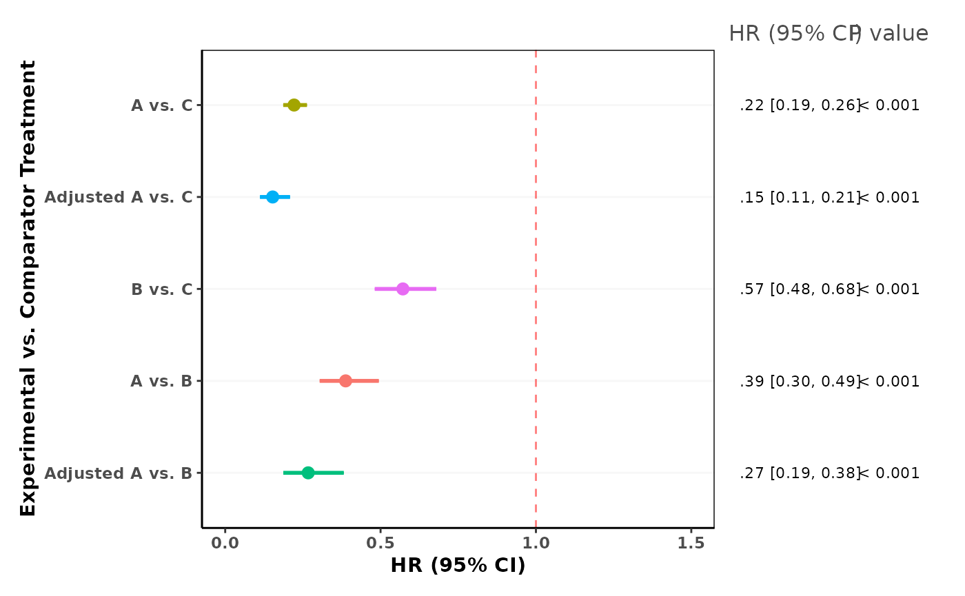
## [1] NAVisualizing effect estimates with forest plot
We can use maic_forest_plot() function to visualize the effect estimates and their confidence intervals from an anchored MAIC object. If bootstrapped confidence intervals exist, these will be displayed. Otherwise, the standard confidence intervals from the summary will be used.
maic_forest_plot(
  result,
  xlim = c(0, 1.5), # Default, can adjust x-axis limits as appropriate for your HR/OR/RR range
  reference_line = 1 # Default, can adjust to be consistent with HR/OR/RR
)